An Overview of IAMR Code

IAMR is built upon the AMReX C++ framework. This provides high-level classes for managing an adaptive mesh refinement simulation, including the core data structures required in AMR calculations. Since IAMR leaverages heavily from the AMReX library, it’s documentation Welcome to AMReX’s documentation is a useful resource in addition to this User’s Guide.

The IAMR simulation begins in IAMR/Source/main.cpp where an instance of the AMReX Amr class is created:

Amr* amrptr = new Amr;

The initialization, including calling a problem’s initdata() routine and refining the base grid occurs next through

amrptr->init(strt_time,stop_time);

And then comes the main loop over coarse timesteps until the desired simulation time is reached:

while ( amrptr->okToContinue()                            &&
       (amrptr->levelSteps(0) < max_step || max_step < 0) &&
       (amrptr->cumTime() < stop_time || stop_time < 0.0) )

{
   //
   // Do a timestep.
   //
   amrptr->coarseTimeStep(stop_time);
}

This uses the AMReX machinery to do the necessary subcycling in time, including synchronization between levels, to advance the level hierarchy forward in time.

State Data

The StateData class structure defined by AMReX is the data container used to store the field data associated with the state on a single AMR level during an IAMR run. The entire state consists of a dynamic union, or hierarchy, of nested StateData objects. Periodic regrid operations modify the hierarchy, changing the shape of the data containers at the various levels according to user-specified criteria; new StateData objects are created for the affected levels, and are filled with the “best” (finest) available data at each location. Instructions for building and managing StateData are encapsulated in the AMReX class, StateDescriptor; as discussed later, a StateDescriptor will be created for each type of state field, and will include information about data centering, required grow cells, and instructions for transferring data between AMR levels during various synchronization operations.

In IAMR/Source/NavieStokesBase.H, the enum StateType defines the different state descriptors for IAMR. These are setup during the run by code in NS_setup.cpp, and include (but are not limited to):

State_Type: the cell-centered density, velocity, and other scalars (tracers)
Press_Type: the node-centered dynamic pressure field.
Divu_Type: Stores the right-hand-side of the constraint (only matters for low Mach flows when this is nonzero).
Dsdt_Type: Stores the time-derivative of the right-hand-side of the constraint (only matters for low Mach flows when this is nonzero).

Each StateData object has two MultiFabs, one each for old and new times, and can provide an interpolated copy of the state at any time between the two. Alternatively, can also access the data containers directly, for instance:

MultiFab& S_new = get_new_data(State_Type);

gets a pointer to the multifab containing the hydrodynamics state data at the new time (here State_Type is the enum defined in NavierStokesBase.H) (note that the class NavierStokes is a derived classes of NavierStokesBase).

MultiFab data is distributed in space at the granularity of each Box in its BoxArray. We iterate over MultiFabs using a special iterator, MFIter, which knows about the locality of the data—only the boxes owned by the processor will be included in the loop on each processor. An example loop (taken from code in NavierStokesBase.cpp):

//
// Fill rho at half time
//
#ifdef _OPENMP
#pragma omp parallel if (Gpu::notInLaunchRegion())
#endif
    for (MFIter mfi(rho_half,TilingIfNotGPU()); mfi.isValid(); ++mfi)
    {
        const Box& bx = mfi.growntilebox();

        // half time
        auto const& rho_h = rho_half.array(mfi);
        // previous time
        auto const& rho_p = rho_ptime.array(mfi);
        // current time
        auto const& rho_c = rho_ctime.array(mfi);

        amrex::ParallelFor(bx, [rho_h, rho_p, rho_c]
        AMREX_GPU_DEVICE(int i, int j, int k) noexcept
        {
           rho_h(i,j,k) = 0.5 * (rho_p(i,j,k) + rho_c(i,j,k));
        });
    }
}

Here, ++mfi iterates to the next FArrayBox owned by the MultiFab, and mfi.isValid() returns false after we’ve reached the last box contained in the MultiFab, terminating the loop. rho_half.array(mfi) creates an object for accessing FArrayBox data in a more array like manner using operator() (more details are in the AMReX documentation at https://amrex-codes.github.io/amrex/docs_html/Basics.html#sec-basics-array4 ).

Here ParallelFor takes two arguments. The first argument is a Box specifying the iteration index space, and the second argument is a C++ lambda function that works on cell (i,j,k). Variables rho_half, rho_ptime and rho_ctime in the lambda function are captured by value from the enclosing scope. The code above is performance portable. It works with and without GPU support. When IAMR is built with GPU support (USE_CUDA=TRUE), AMREX_GPU_DEVICE indicates that the lambda function is a device function and ParallelFor launches a GPU kernel to do the work. When it is built without GPU support, AMREX_GPU_DEVICE has no effects whatsoever. It should be emphasized that ParallelFor does not start an OpenMP parallel region. The OpenMP parallel region will be started by the pragma above the MFIter loop if it is built with OpenMP and without enabling GPU (USE_OMP=TRUE and USE_CUDA=TRUE are not compatible). Tiling is turned off if GPU is enabled so that more parallelism is exposed to GPU kernels. Also note that when tiling is off, tilebox returns validbox. (more details are in the AMReX documentation at https://amrex-codes.github.io/amrex/docs_html/GPU.html#sec-gpu-for ).

Boundaries

In AMReX, we are primarily concerned with enabling structured-grid computations. A key aspect of this is the use of “grow” cells around the “valid box” of cells over which we wish to apply stencil operations. Grow cells, filled properly, are conveniently located temporary data containers that allow us to separate the steps of data preparation (including communication, interpolation, or other complex manipulation) from stencil application. The steps that are required to fill grow cells depends on where the cells “live” in the computational domain.

Boundaries Between Grids and Levels

Most of our state data is cell-centered, and often the grow cells are as well. When the cells lie directly over cells of a neighboring box at the same AMR refinement level, these are “fine-fine” cells, and are filled by direct copy (including any MPI communication necessary to enable that copy). Note that fine-fine boundary also include grow cells that cover valid fine cells through a periodic boundary.

When the boundary between valid and grow cells is coincident with a coarse-fine boundary, these coarse-fine grow cells will hold cell-centered temporary data that generated by interpolation (in space and time) of the underlying coarse data. This operation requires auxiliary metadata to define how the interpolation is to be done, in both space and time. Importantly, the interpolation also requires that coarse data be well-defined over a time interval that brackets the time instant for which we are evaluating the grow cell value – this places requirements on how the time-integration of the various AMR levels are sequenced relative to eachother. In AMReX, the field data associated with the system state, as well as the metadata associated with inter-level transfers, is bundled (encapsulated) in a class called “StateData”. The metadata is defined in NS_setup.cpp – search for cell_cons_interp, for example – which is “cell conservative interpolation”, i.e., the data is cell-based (as opposed to node-based or edge-based) and the interpolation is such that the average of the fine values created is equal to the coarse value from which they came. (This wouldn’t be the case with straight linear interpolation, for example.) A number of interpolators are provided with AMReX and user-customizable ones can be added on the fly.

Physical Boundaries

The last type of grow cell exists at physical boundaries. These are special for a couple of reasons. First, the user must explicitly specify how they are to be filled, consistent with the problem being run. AMReX provides a number of standard condition types typical of PDE problems (reflecting, extrapolated, etc), and a special one that indicates external Dirichlet. In the case of Dirichlet, the user supplies data to fill grow cells.

IAMR provides the ability to specify constant Dirichlet BCs in the inputs file (see section Dirichlet Boundary Conditions). Users can create more complex Dirichlet boundary condtions by writing their own fill function in NS_bcfill.H, then using that function to create an amrex::StateDescriptor::BndryFunc object and specifying which variables will use it in NS_setup.cpp.

It is important to note that external Dirichlet boundary data is to be specified as if applied on the face of the cell bounding the domain, even for cell-centered state data. For cell-centered data, the array passed into the boundary condition code is filled with cell-centered values in the valid region and in fine-fine, and coarse-fine grow cells. Additionally, grow cells for standard extrapolation and reflecting boundaries are pre-filled. The differential operators throughout IAMR are aware of the special boundaries that are Dirichlet and wall-centered, and the stencils are adjusted accordingly.

For convenience, IAMR provides a limited set of mappings from a physics-based boundary condition specification to a mathematical one that the code can apply. This set can be extended by adjusting the corresponding translations in NS_BC.H, but, by default, includes (See AMReX/Src/Base/AMReX_BC_TYPES.H for more detail):

Outflow:
- velocity: FOEXTRAP
- temperature: FOEXTRAP
- scalars: FOEXTRAP
No Slip Wall with Adiabatic Temp:
- velocity: EXT_DIR, \(u=v=0\)
- temperature: REFLECT_EVEN, \(dT/dt=0\)
- scalars: HOEXTRAP
Slip Wall with Adiabatic Temp:
- velocity: EXT_DIR, \(u_n=0\); HOEXTRAP, \(u_t\)
- temperature: REFLECT_EVEN, \(dT/dn=0\)
- scalars: HOEXTRAP

The keywords used above are defined:

INT_DIR: data taken from other grids or interpolated
EXT_DIR: data specified on EDGE (FACE) of bndry
HOEXTRAP: higher order extrapolation to EDGE of bndry
FOEXTRAP: first order extrapolation from last cell in interior
REFLECT_EVEN: \(F(-n) = F(n)\) true reflection from interior cells
REFLECT_ODD: \(F(-n) = -F(n)\) true reflection from interior cells

Derived Variables

IAMR has the ability to created new variables derived from the state variables. A few derived variables are provided with IAMR, which can be used as examples for creating user defined derived variables. Users create derived variables by adding a function to create them in NS_derive.H and NS_derive.cpp, and then adding the variable to the derive_lst in NS_setup.cpp.

Access to the derived variable is through one of two amrex:AmrLevel functions (which are inherited by NavierStokesBase and NavierStokes):

/**
* \brief Returns a MultiFab containing the derived data for this level.
* The user is responsible for deleting this pointer when done
* with it.  If ngrow>0 the MultiFab is built on the appropriately
* grown BoxArray.
*/
virtual std::unique_ptr<MultiFab> derive (const std::string& name,
                      Real               time,
                      int                ngrow);
/**
* \brief This version of derive() fills the dcomp'th component of mf
* with the derived quantity.
*/
virtual void derive (const std::string& name,
                     Real               time,
                     MultiFab&          mf,
                     int                dcomp);

As an example, mag_vort is a derived variable provided with IAMR, which returns the magnitude of the vorticity of the flow. A multifab filled with the magnitude of the vorticity can be obtained via

std::unique_ptr<MultiFab> vort;
vort = derive(mag_vort, time, ngrow);
//
// do something with vorticity...
//
vort.reset();

The FillPatchIterator

A FillPatchIterator is a AMReX object tasked with the job of filling rectangular patches of state data, possibly including grow cells, and, if so, utilizing all the metadata discussed above that is provided by the user. Thus, a FillPatchIterator can only be constructed on a fully registered StateData object, and is the preferred process for filling grown platters of data prior to most stencil operations (e.g., explicit advection operators, which may require several grow cells). It should be mentioned that a FillPatchIterator fills temporary data via copy operations, and therefore does not directly modify the underlying state data. In the code, if the state is modified (e.g., via an advective “time advance”, the new data must be copied explicitly back into the StateData containers.

Use of FillPatchIterator as an iterator has been depreciated in favor of MFIter, which supports tiling (see section Parallelization). However, IAMR continues to use FillPatchIterator for creating temporaries with filled grow cells.

For example, the following code demonstrates the calling sequence to create and use a FillPatchIterator for preparing a rectangular patch of data that includes the “valid region” plus NUM_GROW grow cells. Here, the valid region is specified as a union of rectangular boxes making up the box array underlying the MultiFab S_new, and NUM_GROW cells are added to each box in all directions to create the temporary patches to be filled.

FillPatchIterator fpi(*this, S_new, NUM_GROW,
                      time, State_Type, strtComp, NUM_STATE);
// Get a reference to the temporary platter of grown data
MultiFab& S = fpi.get_mf();

Here the FillPatchIterator fills the patch with data of type “State_Type” at time “time”, starting with component strtComp and including a total of NUM_STATE components. When the FillPatchIterator goes out of scope, it and the temporary data platters are destroyed (though much of the metadata generated during the operation is cached internally for performance). Notice that since NUM_GROW can be any positive integer (i.e., that the grow region can extend over an arbitrary number of successively coarser AMR levels), this key operation can hide an enormous amount of code and algorithm complexity.

Parallelization

AMReX uses a hybrid MPI + X approach to parallelism, where X = OpenMP for multicore machines, and CUDA/HIP/DCP++ for CPU/GPU systems. The basic idea is that MPI is used to distribute individual boxes across nodes while X is used to distribute the work in local boxes within a node. The OpenMP approach in AMReX is optionally based on tiling the box-based data structures. Both the tiling and non-tiling approaches to work distribution are discussed below. Also see the discussion of tiling in AMReX’s documentation, MFIter and Tiling.

AMReX’s Non-Tiling Approach

At the highest abstraction level, we have MultiFab (mulitple FArrayBoxes). A MultiFab contains an array of Boxes (a Box contains integers specifying the index space it covers), including Boxes owned by other processors for the purpose of communication, an array of MPI ranks specifying which MPI processor owns each Box, and an array of pointers to FArrayBoxes owned by this MPI processor. A typical usage of MultiFab is as follows,

for (MFIter mfi(mf); mfi.isValid(); ++mfi) // Loop over boxes
{
  // Get the index space of this iteration
  const Box& box = mfi.validbox();

  // Get a reference to mf's data as a multidimensional array
  auto& data = mf.array(mfi);

  // Loop over "box" to update data.
  // On CPU/GPU systems, this loop executes on the GPU
}

A few comments about this code

Here the iterator, mfi, will perform the loop only over the boxes that are local to the MPI task. If there are 3 boxes on the processor, then this loop has 3 iterations.
box as returned from mfi.validbox() does not include ghost cells. We can get the indices of the valid zones as box.loVect and box.hiVect.

AMReX’s Tiling Approach

There are two types of tiling that people discuss. In logical tiling, the data storage in memory is unchanged from how we do things now in pure MPI. In a given box, the data region is stored contiguously). But when we loop in OpenMP over a box, the tiling changes how we loop over the data. The alternative is called separate tiling—here the data storage in memory itself is changed to reflect how the tiling will be performed. This is not considered in AMReX.

In our logical tiling approach, a box is logically split into tiles, and a MFIter loops over each tile in each box. Note that the non-tiling iteration approach can be considered as a special case of tiling with the tile size equal to the box size.

bool tiling = true;
for (MFIter mfi(mf,tiling); mfi.isValid(); ++mfi) // Loop over tiles
{
  // Get the index space of this iteration
  const Box& box = mfi.tilebox();

  // Get a reference to mf's data as a multidimensional array
  auto& data = mf.array(mfi);

  // Loop over "box" to update data.
}

Note that the code is almost identical to the one with the non-tiling approach. Some comments:

The iterator now takes an extra argument to turn on tiling (set to true). There is another interface fo MFIter that can take an IntVect that explicitly gives the tile size in each coordinate direction.

If we don’t explictly specify the tile size at the loop, then the runtime parameter fabarray.mfiter_tile_size can be used to set it globally.
.validBox() has the same meaning as in the non-tile approach, so we don’t use it. Instead, we use .tilebox() to get the Box (and corresponding lo and hi) for the current tile, not the entire data region.

Let us consider an example. Suppose there are four boxes:

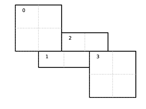
A simple domain showing 4 Boxes labeled 0–3, and their tiling regions (dotted lines) — Fig. 8 Boxes labeled 0–3, and their tiling regions (dotted lines)

The first box is divided into 4 logical tiles, the second and third are divided into 2 tiles each (because they are small), and the fourth into 4 tiles. So there are 12 tiles in total. The difference between the tiling and non-tiling version are then:

In the tiling version, the loop body will be run 12 times. Note that tilebox is different for each tile, whereas fab might be referencing the same object if the tiles belong to the same box.
In the non-tiling version (by constructing MFIter without the optional second argument or setting to false), the loop body will be run 4 times because there are four boxes, and a call to mfi.tilebox() will return the traditional validbox. The non-tiling case is essentially having one tile per box.

Tiling provides us the opportunity of a coarse-grained approach for OpenMP. Threading can be turned on by inserting the following line above the for (MFIter…) line.

#pragma omp parallel

Assuming four threads are used in the above example, thread 0 will work on 3 tiles from the first box, thread 1 on 1 tile from the first box and 2 tiles from the second box, and so forth. Note that OpenMP can be used even when tiling is turned off. In that case, the OpenMP granularity is at the box level (and good performance would need many boxes per MPI task).

While it is possible that, independent of whether or not tiling is on, OpenMP threading could also be started within the function/loop called inside the MFIter loop, rather than at the MFIter loop level, this is not the approach taken in IAMR.

The tile size for the three spatial dimensions can be set by a parameter, e.g., fabarray.mfiter_tile_size = 1024000 8 8. A huge number like 1024000 will turn off tiling in that direction. As noted above, the MFIter constructor can also take an explicit tile size: MFIter(mfi(mf,IntVect(128,16,32))).

Note that tiling can naturally transition from all threads working on a single box to each thread working on a separate box as the boxes coarsen (e.g., in multigrid).

The MFIter class provides some other useful functions:

mfi.validbox()       : The same meaning as before independent of tiling.
mfi.growntilebox(int): A grown tile box that includes ghost cells at box
                       boundaries only.  Thus the returned boxes for a
                       Fab are non-overlapping.
mfi.nodaltilebox(int): Returns non-overlapping edge-type boxes for tiles.
                       The argument is for direction.
mfi.fabbox()         : Same as mf[mfi].box().

Finally we note that tiling is not always desired or better. This traditional fine-grained approach coupled with dynamic scheduling is more appropriate for work with unbalanced loads, such as chemistry burning in cells by an implicit solver. Tiling can also create extra work in the ghost cells of tiles.

Practical Details in Working with Tiling

It is the responsibility of the coder to make sure that the routines within a tiled region are safe to use with OpenMP. In particular, note that:

tile boxes are non-overlapping
the union of tile boxes completely cover the valid region of the fab
Consider working with a node-centered MultiFab, s_nd, and a cell-centered MultiFab, s_cc:
- with mfi(s_cc), the tiles are based on the cell-centered index space. If you have an \(8\times 8\) box, then and 4 tiles, then your tiling boxes will range from \(0\rightarrow 3\), \(4\rightarrow 7\).
- with mfi(s_nd), the tiles are based on nodal indices, so your tiling boxes will range from \(0\rightarrow 3\), \(4\rightarrow 8\).
When updating routines to work with tiling, we need to understand the distinction between the index-space of the entire box (which corresponds to the memory layout) and the index-space of the tile. Inside the MFIter loop, make sure to only update over the tile region, not for the entire box.

Particles

IAMR has the ability to include data-parallel particle simulations. Our particles can interact with data defined on a (possibly adaptive) block-structured hierarchy of meshes. Example applications include Particle-in-Cell (PIC) simulations, Lagrangian tracers, or particles that exert drag forces onto a fluid, such as in multi-phase flow calculations.

Within IAMR, we provide an example of passively advected tracer particles in IAMR/Tutorials/Particles.

We provide a brief introduction to using particles in IAMR in Creating and Running Your Own Problem. For more detailed information on particles, see AMReX’s documentation: Particles.

Gridding and Load Balancing

IAMR has a great deal of flexibility when it comes to how to decompose the computational domain into individual rectangular grids, and how to distribute those grids to MPI ranks. There can be grids of different sizes, more than one grid per MPI rank, and different strategies for distributing the grids to MPI ranks. IAMR relies on AMReX for the implementation. For more information, please see AMReX’s documentation, found here: Gridding and Load Balancing.

See AMR Grids and Gridding and Load Balancing for how grids are created, i.e. how the BoxArray on which MultiFabs will be built is defined at each level.

See Load Balancing for the strategies AMReX supports for distributing grids to MPI ranks, i.e. defining the DistributionMapping with which MultiFabs at that level will be built.

When running on multicore machines with OpenMP, we can also control the distribution of work by setting the size of grid tiles (by defining fabarray.mfiter_tile_size, see Tiling). We can also specify the strategy for assigning tiles to OpenMP threads. See Parallelization and AMReX’s docmumentation (MFIter with Tiling) for more about tiling.

AMR Grids

Our approach to adaptive refinement in IAMR uses a nested hierarchy of logically-rectangular grids with simultaneous refinement of the grids in both space and time. The integration algorithm on the grid hierarchy is a recursive procedure in which coarse grids are advanced in time, fine grids are advanced multiple steps to reach the same time as the coarse grids and the data at different levels are then synchronized.

During the regridding step, increasingly finer grids are recursively embedded in coarse grids until the solution is sufficiently resolved. An error estimation procedure based on user-specified criteria (described in Tagging for Refinement) evaluates where additional refinement is needed and grid generation procedures dynamically create or remove rectangular fine grid patches as resolution requirements change.

The dynamic creation and destruction of grid levels is a fundamental part of IAMR’s capabilities. At regular intervals (set by the user), each Amr level that is not the finest allowed for the run will invoke a “regrid” operation. When invoked, a set of error tagging functions is traversed. For each, a field specific to that function is derived from the state over the level, and passed through a kernel that “set”’s or “clear”’s a flag on each cell. The field and function for each error tagging quantity is identified in the setup phase of the code (in NS_error.cpp). Each function adds or removes to the list of cells tagged for refinement. This may then be extended if amr.n_error_buf \(> 0\) to a certain number of cells beyond these tagged cells. This final list of tagged cells is sent to a grid generation routine, which uses the Berger-Rigoutsos algorithm to create rectangular grids which will define a new finer level (or set of levels). State data is filled over these new grids, copying where possible, and interpolating from coarser level when no fine data is available. Once this process is complete, the existing Amr level(s) is removed, the new one is inserted into the hierarchy, and the time integration continues.

Further details on grid generation are in AMReX’s documentation: Grid Creation.

Parallel I/O

Both checkpoint files and plotfiles are actually folders containing subfolders: one subfolder for each level of the AMR hierarchy. The fundamental data structure we read/write to disk is a MultiFab, which is made up of multiple FAB’s, one FAB per grid. Multiple MultiFabs may be written to each folder in a checkpoint file. MultiFabs of course are shared across CPUs; a single MultiFab may be shared across thousands of CPUs. Each CPU writes the part of the MultiFab that it owns to disk, but they don’t each write to their own distinct file. Instead each MultiFab is written to a runtime configurable number of files N (N can be set in the inputs file as the parameter amr.checkpoint_nfiles and amr.plot_nfiles; the default is 64). That is to say, each MultiFab is written to disk across at most N files, plus a small amount of data that gets written to a header file describing how the file is laid out in those N files.

What happens is \(N\) CPUs each opens a unique one of the \(N\) files into which the MultiFab is being written, seeks to the end, and writes their data. The other CPUs are waiting at a barrier for those \(N\) writing CPUs to finish. This repeats for another \(N\) CPUs until all the data in the MultiFab is written to disk. All CPUs then pass some data to CPU 0 which writes a header file describing how the MultiFab is laid out on disk.

We also read MultiFabs from disk in a “chunky” manner, opening only \(N\) files for reading at a time. The number \(N\), when the MultiFabs were written, does not have to match the number \(N\) when the MultiFabs are being read from disk. Nor does the number of CPUs running while reading in the MultiFab need to match the number of CPUs running when the MultiFab was written to disk.

Think of the number \(N\) as the number of independent I/O pathways in your underlying parallel filesystem. Of course a “real” parallel filesytem should be able to handle any reasonable value of \(N\). The value -1 forces \(N\) to the number of CPUs on which you’re running, which means that each CPU writes to a unique file, which can create a very large number of files, which can lead to inode issues.